
Introduction
- LiDAR는 high frequency range measurements를 제공하여 mapping에 흔히 쓰이는 센서이다. 그러나 LiDAR가 이동을 하게되면 정확한 mapping을 위해서는 lidar의 pose가 필요하다. (Solution 1) independent position estimation by GPS/INS, Solution 2) odometry measurements by wheel encoders or visual odometry)
- 성능향상을 위해 SLAM의 복잡한 문제를 분리하여 해결하는 방법을 제안한다.
- Algorithm 1: high frequency에서 odometry 수행
- Algorithm 2: low frequency로 fine matching과 point cloud registration 수행
Software System Overview
- P^hat: laser scan으로 얻어진 points
- P_k: k sweep동안 결합된 point cloud를 의미하며 이는 Lidar Odometry algorithm과 Lidar Mapping에서 활용된다.
- Lidar Odometry (10Hz): point cloud는 두개의 연속적인 sweep에 대한 lidar motion 계산에 쓰인다. 추정된 motion은 P_k의 distortion 보정에 사용된다. -> publish pose transforms
- Lidar Mapping (1Hz): undistorted P_k는 map상에 match 및 register된다. -> publish pose transforms
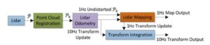
=> 두 알고리즘에 의한 pose transforms은 통합되어 transform output을 생산한다.
LiDAR ODOMETRY (Feature Point Extraction)
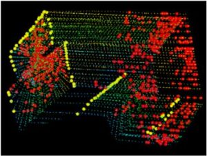
- LiDAR cloud P_k로 부터 feature points를 추출한다.
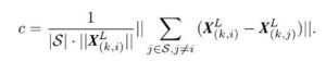
- smoothness c (of the local surface): threshold를 기준으로 c가 크면 edge <-> c가 작으면 planar
- Fig 2에서 yellow: edge, red: planar
Finding Feature Point Correspondence
- Odometry Algorithm: 한 sweep내에서 lidar의 motion 추정
- P_k bar: t_k+1시점에서 reproject된 P_k를 의미한다. 이는 새롭게 얻어진 P_k+1과 함께 lidar motion 추정에 활용된다.
- Correspondence: P_k bar와 P_k+1를 가지고 두 lidar cloud간의 correspondence를 찾는다. 이때, epsilon_k+1과 H_k+1은 각각 P_k+1에서 얻은 edge point와 planar point를 의미한다. 그리고 P_k bar에서는 epsilon_k+1과 H_k+1에 상응하는 edge line과 planar patch를 찾는다. 그리고 매 iteration마다 epsilon_k+1과 H_k+1은 추정된 transform을 통해 sweep 시작점에 reproject된다. 그리고 이는 epsilon_k+1 ~, H_k+1 ~로 표기된다.
- 그리고 P_k bar에서 ~에 가장 가까운 point를 찾는다.
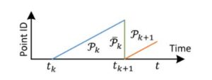
- Correspondence와 현재 feature (i)간의 distance 정의가 필요하다. 보통은 Euclidean distance를 활용하지만, 여기서 feature point가 정확히 같은 위치에서 추출된 것이 아니라 Edge distance를 사용한다.


Notation
- t: current time stamp
- t_k+1: sweep k+1의 starting time
- T_k+1^L: [t_k+1, t]사이의 lidar pose transform
Motion Estimation
- 한 sweep내에서 Lidar motion의 constant angular 및 linear velocity 특성을 통해 다른 시간 t에 대한 pose transform을 linear interpolation을 통해 구할 수 있다. 이를통해 [t_k+1, i] 사이 시점에 해당하는 lidar pose transform을 아래와 같이 구할 수 있다.
- 그리고 이렇게 구한 pose transform을 적용하여 i시점의 좌표를 구할 수 있다.
- d를 minimize하는 transform matrix T_k+1^L 을 구하는 것이 motion estimation이다.
![]()
![]()

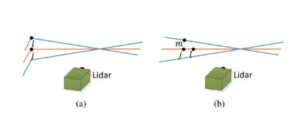
LiDAR Mapping
- T_k^w (blue line): Lidar pose on the map by mapping algorithm
- T_k+1^L(orange line): lidar motion by odometry algorithm.
- Q_k+1 bar (green line): odometry algorithm에 의해 publish된 undistorted point cloud가 map상에 project되고, 기존 map Q_k (black line)과 match된다.
- LiDAR mapping에서도 마찬가지로 feature point를 추출하고, 이들의 correspondence를 찾아 이들간의 distance를 구한다.
- Levenberg-Marquardt (LM) optimization방법으로 pose를 보정한다.

Comment
- LiDAR 한 회전에 얻어지는 데이터를 k, 한 회전안에서 각각을 i, i+1,,,이런식으로 생각해야 한다.
- Odometry를 적용하지 않으면 매우 비효율적일 수 있다. Odometry를 쓰면 Global좌표계에 이어 붙일 때 대략적인 위치에서 optimization을 통해 map을 이어붙이면 된다. 그러나 이를 사용하지 않을 경우, 예를들어 원점에서 부터 시작하여 새로구해진 point cloud를 어떻게 잘 맞게 이어붙일지를 하나하나 해봐야 한다. 이렇게 되면 비용이 훨씬 더 많이 들 수 밖에 없다.